Overview
This overview discusses the basic constituents of the SPiRA framework. This includes how data from the fabrication process is connected to the design environment, the basic design template for creating parameterized cells, and how different layout elements are defined.
Process Design Kit
The process design kit (PDK) is a set of technology files needed to implement the physical aspects of a layout design. Application-specific rules specified in the PDK controls how physical design applications work.
A new PDK scheme is introduced. The Python programming language is used to bind PDK data to a set of classes, called data trees, that uniquely categorises PDK data. This new PDK scheme is called the Rule Deck Database (RDD), also refered to as the Rule Design Database. By having a native PDK in Python it becomes possible to use methods from the SPiRA framework to create a more descriptive PDK database. A design process typically contains the following aspects:
- GDSII Data: Contains general settings required by the GDSII library, such as grid size.
- Process Data: Contains the process layers, layer purposes, layer parameters, and layer mappings.
- Virtual Modelling: Define derived layers that describes layer boolean operations.
Initialization
All caps are used to represent the RDD syntax. The reason being to make the script structure clearly distinguishable from the rest of the framework source code. First, the RDD object is initialized, followed by the process name and description, and then the GDSII related variables are defined.
RDD.GDSII = ParameterDatabase()
RDD.GDSII.UNIT = 1e-6
RDD.GDSII.GRID = 1e-12
RDD.GDSII.PRECISION = 1e-9
Process Data
Process data relates to data provided by a specific fabrication technology.
Process Layer
The first step in creating a layer is to define the process step that it represents in mask fabrication. The layer process defines a specific fabrciation function, for examples metalization. There can be multiple different drawing layers for a single process. A process database object is created that contains all the different process steps in a specific fabrication process:
RDD.PROCESS = ProcessLayerDatabase()

RDD.PROCESS.R1 = ProcessLayer(name='Resistor 1', symbol='R1')
RDD.PROCESS.M1 = ProcessLayer(name='Metal 1', symbol='M1')
RDD.PROCESS.C1 = ProcessLayer(name='Contact 1', symbol='C1')
Each process has a name that describes the process function, and a symbol that is used to identify the process.
Purpose Layer
The purpose indicates the use of the layer. Multiple layers with the same process but different purposes can be created. Similar to a process value each purpose contains a name and a unique symbol. Purposes are defined using a purpose database object:
RDD.PURPOSE = PurposeLayerDatabase()

RDD.PURPOSE.METAL = PurposeLayer(name='Polygon metals', symbol='METAL')
RDD.PURPOSE.VIA = PurposeLayer(name='Contact', symbol='VIA')
Process Parameters
Parameters are added to a process by creating a parameter database object that has a key value equal to the symbol of a pre-defined process:
RDD.M1 = ParameterDatabase()
RDD.M1.MIN_SIZE = 0.7
RDD.M1.MAX_WIDTH = 20.0
RDD.M1.J5_MIN_SURROUND = 0.5
RDD.M1.MIN_SURROUND_OF_I5 = 0.5
Any number of variables can be added to the database using the dot operator. The code above defines a set of design parameters for the M1 process.
Physical Layers
Physical Layers are unique to SPiRA and is defined as a layer that has a defined process and purpose. A physical layer (PLayer) defines the different purposes that a single process can be used for in a layout design.
RDD.PLAYER.M1 = PhysicalLayerDatabase()
RDD.PLAYER.C1 = PhysicalLayerDatabase()

RDD.PLAYER.C1.VIA = PhysicalLayer(process=RDD.PROCESS.C1, purpose=RDD.PURPOSE.VIA)
RDD.PLAYER.M1.METAL = PhysicalLayer(process=RDD.PROCESS.M1, purpose=RDD.PURPOSE.METAL)
The code above illustrates that the layer M1 is a metal layer on process M1,
and layer C1 is a contact via on process C1.
Virtual Modelling
Derived Layers are used to define different PLayer boolean operations. They are typically used for virtual modelling and polygon operations, such as merged polygons or polygon holes.
RDD.PLAYER.M1.EDGE_CONNECTED = RDD.PLAYER.M1.METAL & RDD.PLAYER.M1.OUTSIDE_EDGE_DISABLED
The code above defines a derived layer that is generated when a layer with process M1 and
purpose metal overlaps the outside edges of a M1 layer.
Parameters
Designing a generated layout requires modeling its parameters. To create an effective design environment it becomes paramount to define parameter restrictions. SPiRA uses a meta-configuration to define object parameters, which enables the following features:
- Default values can be set to each parameter.
- Documentation for each parameter can be added.
- Parameters can be cached to ensure they aren’t calculated multiple times.
Introduction
Parameters are derived from the spira.Parameter class. The
ParameterInitializer is responsible for storing the parameters of an
instance. To define parameters the class has to inherit from the ParameterInitializer
class. The following code creates a layer object with a number parameter.
import spira.all as spira
class Layer(spira.ParameterInitializer):
    number = spira.Parameter()

>>> layer = Layer(number=9)
>>> layer.number
9
At first glance this may not seem to add any value that Python by default does not already adds. The same example can be generated using native Python:
class Layer(object):
    def __init__(self, number=0):
        self.number = number
The true value of the parameterized framework becomes clear when adding attributes to the parameter, such as the default value, restrictions, preprocess and doc. These attributes allow a parameter to be type-checked and documented.
import spira.all as spira
class Layer(spira.ParameterInitializer):
    number = spira.Parameter(default=0,
                             restrictions=spira.INTEGER,
                             preprocess=spira.ProcessorInt(),
                             doc='Advanced parameter.')
The newly defined parameter has more advanced features that makes for a more powerful design framework:
# The default value of the parameter is 0.
>>> layer = Layer()
>>> layer.number
0

# The parameter can be updated with an integer.
>>> layer.number = 9
>>> layer.number
9

# The string can be preprocessed to an interger.
>>> layer.number = '8'
>>> layer.number
8

# The string cannot be preprocessed and throws an error.
>>> layer.number = 'Hi'
ValueError: invalid literal for int() with base 10: 'Hi'
Default
When defining a parameter the default value can be explicitly set using the default attribute.
This is a simple method of declaring your parameter.
For more complex functionality the default function attribute, fdef_name, can be used.
This attribute defines the name of a class method that will be used to derive the default value of the parameter.
Advantages of this implementation is:
- Logic operations: The default value can be derived from other defined parameters.
- Inheritance: The default value can be overwritten using class inheritance.
import spira.all as spira
class Layer(spira.ParameterInitializer):
    number = spira.Parameter(default=0)
    datatype = spira.Parameter(fdef_name='create_datatype')

    def create_datatype(self):
        return 2 + 3

>>> layer = Layer()
>>> (layer.number, layer.datatype)
(0, 5)
Restrictions
The validity of a parameter value is calculated by the restriction attribute. In certain cases we want to restrict a parameter value to a certain type or range of values, for example:
- Validate that the value has a specific type, such as a via PCell.
- Validate that the value falls between a specified minimum and maximum.
import spira.all as spira
class Layer(spira.ParameterInitializer):
    number = spira.Parameter(default=0, restrictions=spira.RestrictRange(2,5))
The example above restricts the number parameter of the layer to be between 2 and 5:
>>> layer = Layer()
>>> layer.number = 3
3
>>> layer.number = 1
ValueError: Invalid parameter assignment 'number' of cell 'Layer' with value '1', which is not compatible with 'Range Restriction: [2, 5)'.
Preprocessors
The preprocess attribute converts a received value before assigning it to the parameter. Preprocessors are typically used to convert a value of invalid type to one of a valid type, such as converting a float to an integer.
import spira.all as spira
class Layer(spira.ParameterInitializer):
    number = spira.Parameter(default=0, preprocess=spira.ProcessorInt())

>>> layer = Layer()
>>> layer.number = 1
1
>>> layer.number = 2.1
2
>>> layer.number = 'Hi'
ValueError: invalid literal for int() with base 10: 'Hi'
Documentation
Documentation can be added to the parameter using the doc attribute.
The created class can also be documented using triple qoutation marks.
import spira.all as spira
class Layer(spira.ParameterInitializer):
    """ This is a layer class. """
    number = spira.Parameter(default=0, doc='Parameter documentation.')

>>> layer = Layer()
>>> layer.number
0
>>> layer.__doc__
This is a layer class.
>>> layer.number.__doc__
Parameter documentation.
Cache
SPiRA automatically caches parameters once they have been initialized.
When using class methods to define default parameters using the fdef_name attribute, the value is stored when called for the first time.
Calling this value for the second time will not lead to a re-calculation, but rather the value will be retrieved from the cached dictionary.
The cache is automatically cleared when any parameter in the instance is updated, since other parameters might be dependent on the changed parameters.
Parameterized Cells
GDSII layouts encapsulate element design in the visual domain. Parameterized cells encapsulates elements in the programming domain, and utilizes this domain to map external data to elements. This external data can be data from the PDK or values extracted from an already designed layout using simulation software, such as InductEx. The SPiRA framework uses a scripting framework approach to connect the visual domain with a programming domain. The implemented architecture of SPiRA mimics the physical layout patterns implicit in hand-designed layouts. This framework architecture evolved by developing code heuristics that emerged from the process of creating a PCell.
Creating a PCell is done by defining the elements and parameters required to create the desired layout. The relationship between the elements and parameters are described in a template format. Template design is an innate feature of parameterizing cell layouts. This heuristic concludes to develop a framework to effectively describe the different constituents of a PCell, rather than developing an API. The SPiRA framework was built from the following concepts:
1. Defining Element Shapes This step defines the geometrical shapes from which an element polygon is generated.
The supported shapes are rectangles, triangles, circles, as well as regular and irregular polygons.
Each of these shapes has a set of parameters that control the pattern dimensions, e.g. the parameterized rectangle has two parameters, width and length, that defines its length and width, respectively.
2. Element Shape Transformations This step describes the relation between the elements through a set of operations, that includes transformations of a shape in the x-y plane. Transforming an element involves: movement with a specific offset relative to its original location, rotation of a shape around its center with a specific angle, reflection of a shape around a idefined line, and aligning a shape to another shape with a specific offset and angle.
3. PDK Binding The final step is binding data from the PDK to each created pattern. In SPiRA, process related data is defined in the RDD. From this database the required data can be linked to any specific pattern by defining parameters and their design restrictions.
Shapes
A shape is a basic 2-dimentional geometric pattern that consists of a list of points. These points can be manipulated and transformed as required by the designer, before commiting it to a layout cell.
class ShapeExample(spira.Cell):

    def create_points(self, points):
        points = [[0, 0], [2, 2], [2, 6], [-6, 6], [-6, -6], [-4, -4], [-4, 4], [0, 4]]
        return points
You can create your own shape by creating a class that inherits from spira.Shape.
The shape coordinates are calculated by the create_points class method that is innate to any spira.Shape derived instance.
The spira.Shape class offers a rich set of methods for basic and advanced shape manipulation:
>>> shape = ShapeExample()
>>> shape.points
[[0, 0], [2, 2], [2, 6], [-6, 6], [-6, -6], [-4, -4], [-4, 4], [0, 4]]
>>> shape.area
88
>>> shape.move((10, 0))
[[10, 0], [12, 2], [12, 6], [4, 6], [4, -6], [6, -4], [6, 4], [10, 4]]
>>> shape.x_coords
[10 12 12  4  4  6  6 10]
Elements
The purpose of elements are to wrap geometry data with GDSII layout data. In SPiRA the following elements are defined:
- Polygon: Connects a shape object with layout data (layer number, datatype).
- Label: Generates text data in a GDSII layout.
- SRef: A structure references, or sometimes called a cell reference, refers to another cell object, but with difference transformations.
There are other special objects, called element groups that can be used in the design environment. These objects are mainly a combination of polygons and relations between polygons. These special objects are referenced as if they represent a single shape, and its outline is determined by its bounding box dimensions. The following element groups are defined in the SPiRA framework:
- Cells: Is the most generic group that binds different parameterized elements or clusters, while conserving the geometrical relations between these polygons or clusters.
- Group: A set of elements can be grouped in a logical container.
- Ports: A port is simply a polygon with a label on a dedicated process layer. Typically, port elements are placed on conducting metal layers.
- Routes: A route is defined as a cell that consists of a polygon element and a set of edge ports, that resembles a path-like structure.
The SPiRA design environment for creating a PCEll is broken down into the following basic templated steps:
class PCell(spira.Cell):
    """ My first parameterized cell. """

    # Define parameters here
    number = spira.IntegerParameter(default=0, doc='Parameter example number.')

    def create_elements(self, elems):
        # Define elements here.
        return elems

    def create_ports(self, ports):
        # Define ports here.
        return ports
The most basic SPiRA template to generate a PCell is shown above, and consists of three parts:
- Create a new cell by inheriting from
spira.Cell. This connects the class to the SPiRA framework when constructed. - Define the PCell parameters as class attributes.
- Elements and ports are defined in the
create_elementsandcreate_portsclass methods, which is automatically added to the cell instance. The create methods are special SPiRA class methods that specify how the parameters are used to create the cell.
class PolygonExample(spira.Cell):

    def create_elements(self, elems):
        pts = [[0, 0], [2, 2], [2, 6], [-6, 6], [-6, -6], [-4, -4], [-4, 4], [0, 4]]
        shape = spira.Shape(points=pts)
        elems += spira.Polygon(shape=shape, layer=spira.Layer(1))
        return elems

>>> D = PolygonExample()
>>> D.gdsii_output()

The code above illustrates the creation of a polygon object, using the already defined shape.
The polygon object connects the shape to a GDSII library with a GDSII layer number equal to \(1\).
Once the polygon has been created it can be added to the cell instance using the + operator
to increment the elems list.
Group
Groups are used to apply an operation on a set of polygons, such a retrieving their combined bounding box.
The following example illistrated the use of spira.Group to generate a metal bounding box
around a set of polygons:
class GroupExample(spira.Cell):

    def create_elements(self, elems):

        group = spira.Group()
        group += spira.Rectangle(p1=(0,0), p2=(10,10), layer=spira.Layer(1))
        group += spira.Rectangle(p1=(0,15), p2=(10,30), layer=spira.Layer(1))

        elems += group

        bbox_shape = group.bbox_info.bounding_box(margin=1)
        elems += spira.Polygon(shape=bbox_shape, layer=spira.Layer(2))

        return elems
A group polygon is created around the two defined polygons with a marginal offset of 1 micrometer.
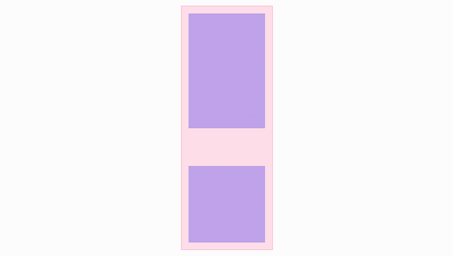
Ports
Port objects are unique to the SPiRA framework and are mainly used for connection purposes.
class Box(spira.Cell):

    width = spira.NumberParameter(default=1)
    height = spira.NumberParameter(default=1)
    layer = spira.LayerParameter(default=spira.Layer(1))

    def create_elements(self, elems):
        shape = shapes.BoxShape(width=self.width, height=self.height)
        elems += spira.Polygon(shape=shape, layer=self.layer)
        return elems

    def create_ports(self, ports):
        ports += spira.Port(name='P1_M1', midpoint=(-0.5,0), orientation=180, width=1)
        ports += spira.Port(name='P2_M1', midpoint=(0.5,0), orientation=0, width=1)
        return ports
>>> box = Box()
[SPiRA: Cell] (name ’Box ’, width 1, height 1, number 0, datatype 0)
>>> box.width
1
>>> box. height
1
>>> box. gds_layer
[SPiRA Layer] (name ’’, number 0, datatype 0)
>>> box.gdsii_output(name='Ports')
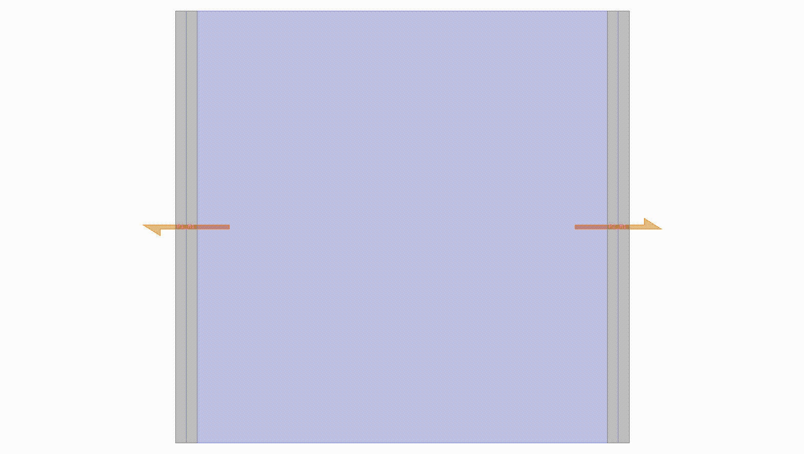
The above example illustrates constructing a parameterized box using the proposed framework:
First, defining the parameters that the user would want to change when creating a box instance.
Here, three parameter are given namely, the width, the height and the layer
properties for GDSII construction. Second, a shape is generated from the defined parameters using the shape module.
Third, this box shape is added as a polygon element to the cell instance. This polygon takes the shape and connects
it to a set of methods responsible for converting it to a GDSII element. Fourth, two terminal ports are added to
the left and right edges of the box, with their directions pointing away from the polygon interior.
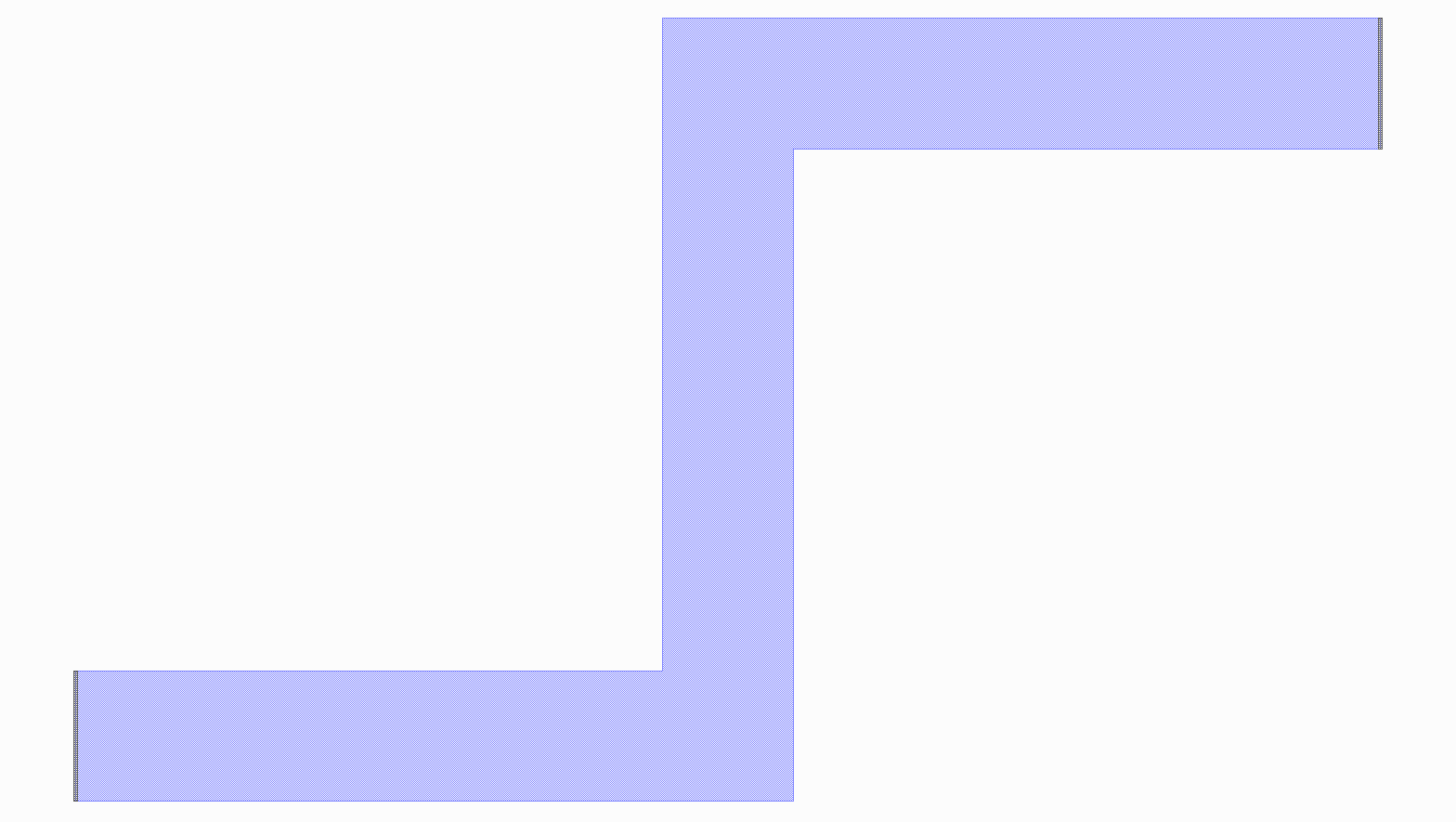
Routes
Most of the times in designing digital electronic circuit layouts it is required to define metal polygon connections between different devices. Defining the exact points connecting different devices can become a tedious task. Routes are polygon classes that automatically generates a polygon path between different devices. As previously explained, ports are used to define connection points to a cell instance. Therefore, routes can be defined as a polygon that connects to two ports through a path-dependent algorithm. SPiRA offers a variety of different route algorithms that can be generated depending on the relative port positions and the user requirements.
class RouteExample(spira.Cell):

    def create_elements(self, elems):
        elems += spira.RouteManhattan(ports=self.ports, layer=spira.Layer(1))
        return elems

    def create_ports(self, ports):
        ports += spira.Port(name='P1', midpoint=(0,0), orientation=180)
        ports += spira.Port(name='P2', midpoint=(20,10), orientation=0)
        return ports
Filters
Filters are algorithms whos state can be toggled (enabled or disabled). These algorithms are typically used to add or remove extra information to an already working design, hence the name filter.
Boolean
Instead of individually looping through the entire tree hierarchy of a layout to apply boolean operations on all polygons, a boolean filter can be used to automate this process.
Layer
Sometimes we want to filter certain layers, since they only serve a temporary purpose, or because we only want to view layers in the design, for example a specific purpose type. In these cases we can use the layer filter to automatically filter certain layers in a cell.
Netlist
The netlist extraction algorithm consists of a chain of filtering methods. The basic algorithmic steps is divided into two categories:
- Extracting a netlist for each individual metal polygon.
- Chaining the metal netlists into a single mask netlist.
For each of these steps there is a chain of filter algorithms applied to ensure the correct extraction:
Polygon Netlist
- Label all nodes in the netlist to the metal layer they represent.
- Label the nodes that are represetative of detected devices.
- Label the nodes that represents ERC connections between differenct metal polygons.
- Calcaulte the cross-over nodes and determine the individual inductive branches.
Mask Netlist
- Combine all metal netlists into a single netlist domain and connect shared nodes.
- Calculate individual branches between device nodes.
- Calculate cross-over nodes between different branches.
- Recalcalate individual branches which includes the detected cross-over nodes.
- Collapse all nodes belonging to the same branch into a single node representation.
RDD Advanced
The goal of the advanced RDD tutorial is to discuss:
- How to define filters.
- How to define derived layers.
- How to create a LVS database.
Filters
Filters leverages the chain of responsiblity design pattern to chain a number of algorithms that has to be executed in a sequential order on a specific layout object.
# First we create a filters database.
RDD.FILTERS = ParameterDatabase()

class PCellFilterDatabase(LazyDatabase):
    """ Define the filters that will be used when creating a spira.PCell object. """

    def initialize(self):
        from spira.yevon import filters

        f = filters.ToggledCompositeFilter(filters=[])
        f += filters.ProcessBooleanFilter(name='boolean', metal_purpose=RDD.PURPOSE.DEVICE_METAL)
        f += filters.SimplifyFilter(name='simplify')
        f += filters.ContactAttachFilter(name='contact_attach')

        f['boolean'] = True
        f['simplify'] = True
        f['contact_attach'] = True

        self.DEVICE = f

        f = filters.ToggledCompositeFilter(filters=[])
        f += filters.ProcessBooleanFilter(name='boolean', metal_purpose=RDD.PURPOSE.CIRCUIT_METAL)
        f += filters.SimplifyFilter(name='simplify')

        f['boolean'] = True
        f['simplify'] = True

        self.CIRCUIT = f

        f = filters.ToggledCompositeFilter(name='mask_filters', filters=[])
        f += filters.ElectricalAttachFilter(name='erc')
        f += filters.PinAttachFilter(name='pin_attach')
        f += filters.DeviceMetalFilter(name='device_metal')

        f['erc'] = True
        f['pin_attach'] = True
        f['device_metal'] = False

        self.MASK = f

RDD.FILTERS.PCELL = PCellFilterDatabase()
The code above shows the creation of three composite filter algorithms:
- The device filters will only be applied on detected device cells.
- The circuit filters will only be aplied on non-device cell.
- The mask filters will be executed on the top-level layout cell.
The PCell filter class inherits from the LazyDatabase class to delay its construction.
Therefore, the PCell filter database is only instantiated when a specific filter is called using
the dot operator as shown below:
f = RDD.FILTERS.PCELL.DEVICE
Derived Layers
Defining derived layers forms the basis of creating the LVS database, since derived layers almost by definition defines via connections.
RDD.VIAS.C5R = ParameterDatabase()

RDD.VIAS.C5R.LAYER_STACK = {
    'BOT_LAYER' : RDD.PLAYER.R5.METAL,
    'TOP_LAYER' : RDD.PLAYER.M6.METAL,
    'VIA_LAYER' : RDD.PLAYER.C5R.VIA
}
RDD.PLAYER.C5R.CLAYER_CONTACT = RDD.PLAYER.R5.METAL & RDD.PLAYER.M6.METAL & RDD.PLAYER.C5R.VIA
RDD.PLAYER.C5R.CLAYER_M1 = RDD.PLAYER.R5.METAL ^ RDD.PLAYER.C5R.VIA
RDD.PLAYER.C5R.CLAYER_M2 = RDD.PLAYER.M6.METAL ^ RDD.PLAYER.C5R.VIA

class C5R_PCELL_Database(LazyDatabase):
    def initialize(self):
        from ..devices.via import ViaC5RA, ViaC5RS
        self.DEFAULT = ViaC5RA
        self.STANDARD = ViaC5RS

RDD.VIAS.C5R.PCELLS = C5R_PCELL_Database()
The example above defines a C5R via which connects layer M6 to R5 through a contact layer C5R. The logic steps for creating this coding snippet is as follow:
- A layer stack is created to defined the top, bottom, and via layers.
- The derived layers are create that specifies the boolean operations between different layers required in order to detect a via connection. Note, that the
RDD.PLAYER.C5R.CLAYER_CONTACTis the via derived layer that specifies the via connection, while the other two derived layers is used for debugging purposes. - A set of different via PCell classes is added to the database. These classes will be constructed and used during the device detection run.
LVS Database
Defining devices in the LVS database is done similarly to defining vias as already explained:
RDD.DEVICES = ParameterDatabase()

RDD.DEVICES.JUNCTION = ParameterDatabase()

class Junction_PCELL_Database(LazyDatabase):
    def initialize(self):
        from ..devices.junction import Junction
        self.DEFAULT = Junction

RDD.DEVICES.JUNCTION.PCELLS = Junction_PCELL_Database()
A Josephson junction device is added to the LVS database by importing an already defined PCell class and can be constucted using the dot operator:
# Create a JTL instance from the definition in the RDD LVS database.
JtlPCell = RDD.DEVICES.JUNCTION.PCELLS.DEFAULT()

# View the created instance.
JtlPCell.gdsii_view()